GIS in R

Background on R

This workshop assumes a basic familiarity with the R programming language and some exposure to GIS concepts like projections.

If you’d like a refresher on R, we suggest the R For Data Science free e-book and the lessons from our beginR workshops, including setup instructions for R and R Studio.

Important packages

Basic packages

As a refresher, in R we install packages from CRAN (The Comprehensive R Archive Network) with the following code:

install.packages(c('tidyverse','scales'))

You’ll only need to install packages once, then you’ll load them into your session with:

library(tidyverse)
library(scales)

We’ll use the tidyverse family of packages to do non-spatial data manipulation today. We’ll use scales to adjust the formatting for some of our maps.

A note on pipes:

Today we’ll use the base R pipe (|>) as our default. You may be more familiar with the magrittr pipe (%>%). The two work very similarly and should usually be interchangeable. If you’d like to use the base R pipe with R Studio’s pipe shortcut (CTRL/CMD + SHIFT + m), you can change the default setting in Tools > Global Options > Code > Use native pipe operator, |> (requires R 4.1+).

Spatial packages

For spatial processing we’ll use the following packages today:

install.packages(c('sf','tidycensus','tigris','arcgislayers','ggmap','ggspatial','basemaps'))

#Spatial processing
library(sf)

#Getting spatial data
library(tidycensus)
library(tigris)
library(arcgislayers)

#Thematic mapping
library(ggmap)
library(ggspatial)
library(basemaps)

The sf packages will be our main spatial processing tool for today.

We’ll explore some of the most common packages for easily loading spatial data: tidycensus for census data, tigris for census boundaries, and arcgislayers for loading data from ESRI Data Services.

Finally we’ll use ggplot from the tidyverse to do some basic mapping and explore extensions with tmap for thematic mapping and ggmap, ggspatial and basemapsfor map annotation, basemaps, and themes.

Resources for R spatial packages:

• Geocomputation with R : general spatial computation in R

• Spatial Data Science: spatial computation with a focus on statistics

• Analyzing US Census Data: tigris and tidycensus

Basic maps

We’ll start of with some basic maps using two very useful packages for retrieving data from Census APIs:

tidycensus and tigris

The tidycensus and tigris packages make it easy to pull census data directly from Census APIs into your R session. tigris pulls TIGER/Line data with boundaries and a few fields (FIPS code, Land and Water Area, etc.) for a variety of census geographies. This is great for various mapping and spatial processing tasks and gives more control over feature resolution.

Sometimes you’ll also want to retrieve census data along with spatial information. tidycensus makes it easy to retrieve tables from a variety of census datasets, along with spatial data when relevant.

Retrieving data

The load_variables function from tidycensus provides a list of the available tables and variables for a given year and census survey, for example 5-year ACS data below:

ac5_vars <- load_variables(year=2024, dataset = "acs5")

We can view the dataset in a separate tab with view(acs5_vars). Note that the early rows are race/ethnicity specific! Let’s load B01001_001, the total population of the tract, to start with.

nc_tracts<- get_acs(geography = "tract", state = "NC", variables = c("B01001_001"),
        output = "wide", geometry = TRUE, year = 2024, cache_table = TRUE,
        progress_bar = FALSE)

Let’s take a look at the data:

nc_tracts |> slice_sample(n=5)

Simple feature collection with 5 features and 4 fields
Geometry type: MULTIPOLYGON
Dimension:     XY
Bounding box:  xmin: -81.64846 ymin: 34.71123 xmax: -76.92791 ymax: 36.41635
Geodetic CRS:  NAD83
        GEOID                                                  NAME B01001_001E
1 37001020302  Census Tract 203.02; Alamance County; North Carolina        3353
2 37195001502     Census Tract 15.02; Wilson County; North Carolina        3266
3 37009970701     Census Tract 9707.01; Ashe County; North Carolina        3829
4 37031970805 Census Tract 9708.05; Carteret County; North Carolina        1773
5 37071030403    Census Tract 304.03; Gaston County; North Carolina        2609
  B01001_001M                       geometry
1         511 MULTIPOLYGON (((-79.40876 3...
2         396 MULTIPOLYGON (((-78.19212 3...
3         527 MULTIPOLYGON (((-81.64749 3...
4         225 MULTIPOLYGON (((-77.13168 3...
5         662 MULTIPOLYGON (((-81.28408 3...

With slice_sample we get random rows from anywhere in the dataset - your results probably look different. This looks like a normal R dataframe except for the additional spatial information at the top and the geometry column. In this case, each entry in the geometry column is a set of points defining a (multi)polygon.

Read more about the geometry types available in sf

# First 10 points of the first feature
as.matrix(nc_tracts$geometry[[1]])[1:10,]

           [,1]     [,2]
 [1,] -79.40216 35.59187
 [2,] -79.40128 35.59396
 [3,] -79.39939 35.59608
 [4,] -79.39812 35.59820
 [5,] -79.39930 35.59951
 [6,] -79.39759 35.60079
 [7,] -79.39695 35.60202
 [8,] -79.39391 35.60383
 [9,] -79.39239 35.60430
[10,] -79.39090 35.60356

Plotting

We can quickly plot sf data with the plot function. We’ll use ggplot to make more complicated maps later on! If you run plot(nc_tracts), every variable will be plotted in a separate map - this can be useful or dangerous depending on your dataset.

plot(nc_tracts['B01001_001E'],border=NA)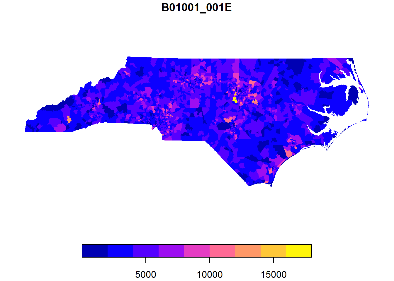

We can also work with sf objects like normal dataframes:

hist(nc_tracts$B01001_001E, breaks = 100)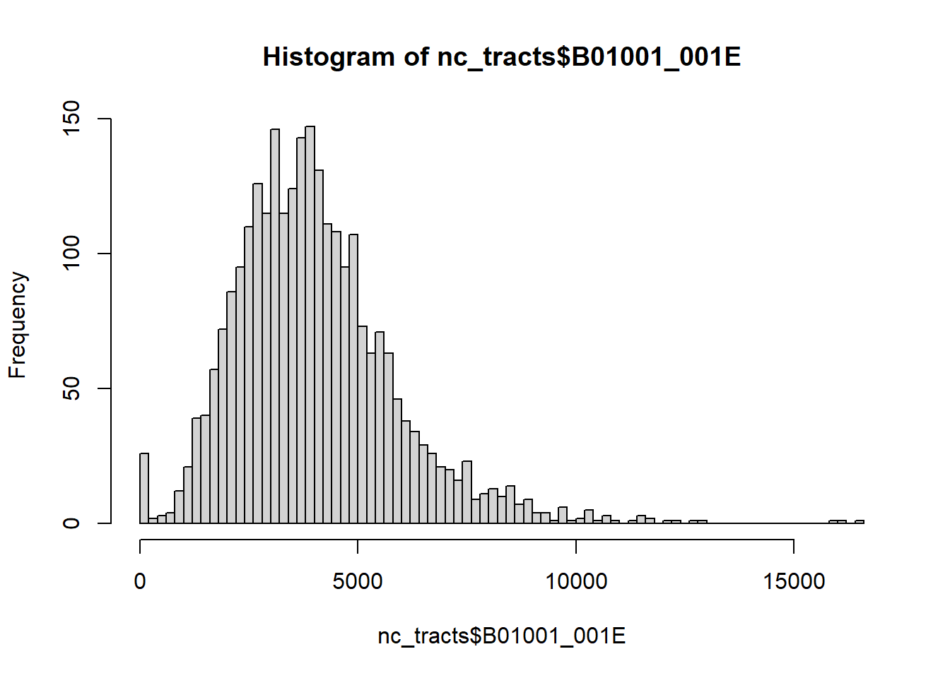

Which tracts are over 15,000 population? We can use dplyr’s filter as usual, but we’ll add an sf function: st_drop_geometry to drop the spatial elements to create a normal dataframe. This will make our output a little more compact (try it without st_drop_geometry!). Removing the geometry can also speed up other operations - it’s worth considering whenever you’re doing more complicated data transformations. You can always use a key variable to rejoin the geometries later on.

Most functions in the sf package start with st_ - we will see many more throughout the workshop.

nc_tracts |> 
  filter(B01001_001E>15000) |> 
  st_drop_geometry()

        GEOID                                             NAME B01001_001E
1 37183053208 Census Tract 532.08; Wake County; North Carolina       16027
2 37183053411 Census Tract 534.11; Wake County; North Carolina       15850
3 37183053428 Census Tract 534.28; Wake County; North Carolina       16415
  B01001_001M
1        1572
2        1495
3        1581

Since all of these tracts are in Wake County, let’s take a closer look at Wake County and the Triangle?

We’ll use the list of counties in the Combined Statistical Area encompassing the Triangle.

tri_counties <- c('37037','37063','37069','37085','37101','37105','37135',
                  '37145','37181', '37183')

tri_tracts <- nc_tracts |> 
  mutate(county_fips = str_sub(GEOID,1,5)) |> 
  filter(county_fips %in% tri_counties)

plot(tri_tracts['B01001_001E'],border = NA)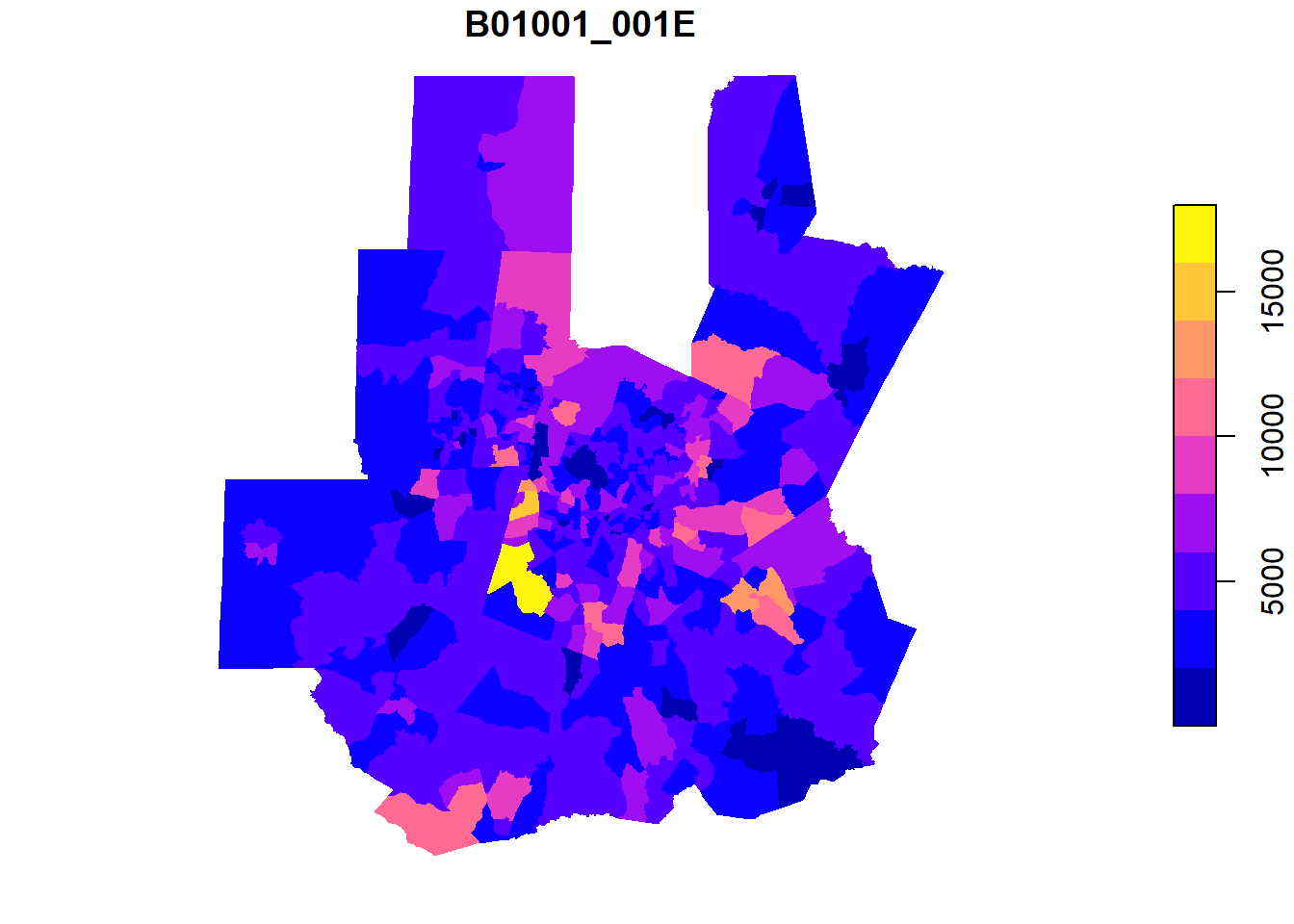

ggplot for mapping

It might be helpful to add the county boundaries to this! Since we don’t need any county data, we can pull county information from tigris with the counties function, then filter to our Triangle counties.

tri_counties <- counties(state="NC", progress_bar = FALSE) |> 
  filter(GEOID %in% tri_counties) 

Retrieving data for the year 2024

Once we start layering data, it’s a good idea to move to ggplot based plots!

ggplot()+
  #color=NA removes borders
  geom_sf(data = tri_tracts, aes(fill = B01001_001E), color=NA)+
  #counties, grey border, no fill color and adjusted linewidth
  geom_sf(data = tri_counties, color = "grey80", fill=NA, lwd = 0.5)+
  scale_fill_viridis_c()+
  theme_minimal()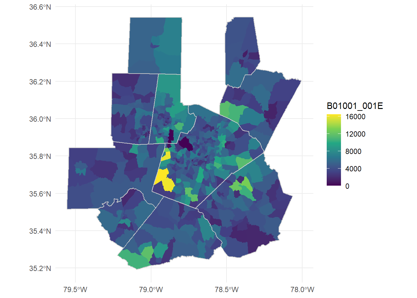

Let’s normalize these tract populations back to their 2020 populations to look directly at growth. We don’t need geometries this time since we’ll join this data to the existing tract boundaries.

acs_vars20 <- load_variables(year=2020, dataset="acs5")

tri_tract_pop_20 <- get_acs(geography = "tract", state = "NC", variables = c("B01001_001"),
        output = "wide", geometry = FALSE, year = 2020, cache_table = TRUE,
        progress_bar = FALSE) |> 
  rename(pop20 = B01001_001E) |> 
  select(GEOID, pop20)

Getting data from the 2016-2020 5-year ACS

tri_tract_chg <- inner_join(tri_tracts, tri_tract_pop_20, by = 'GEOID') |> 
  mutate(pop_change = B01001_001E-pop20,
         pop_change_pct = pop_change/pop20)

The order of the join above is important. Geometries in sf are “sticky” - usually remain in the data with standard dplyr and tidyverse transformations. When we join datasets, the first or left dataset defines whether the result is spatial. Try inner_join(tri_tracts, tri_tract_pop_20, by = 'GEOID') (sf object on the left) and inner_join(``tri_tract_pop_20,``tri_tracts, by = 'GEOID') (sf object on the right) and compare the outputs.

Let’s plot the population changes directly:

ggplot()+
  geom_sf(data = tri_tract_chg, aes(fill = pop_change_pct), color=NA)+
  geom_sf(data = tri_counties, color = "grey80", fill=NA, lwd = 0.5)+
  scale_fill_gradient2(low="red",high="blue", mid="white", labels=scales::percent)+
  theme_minimal()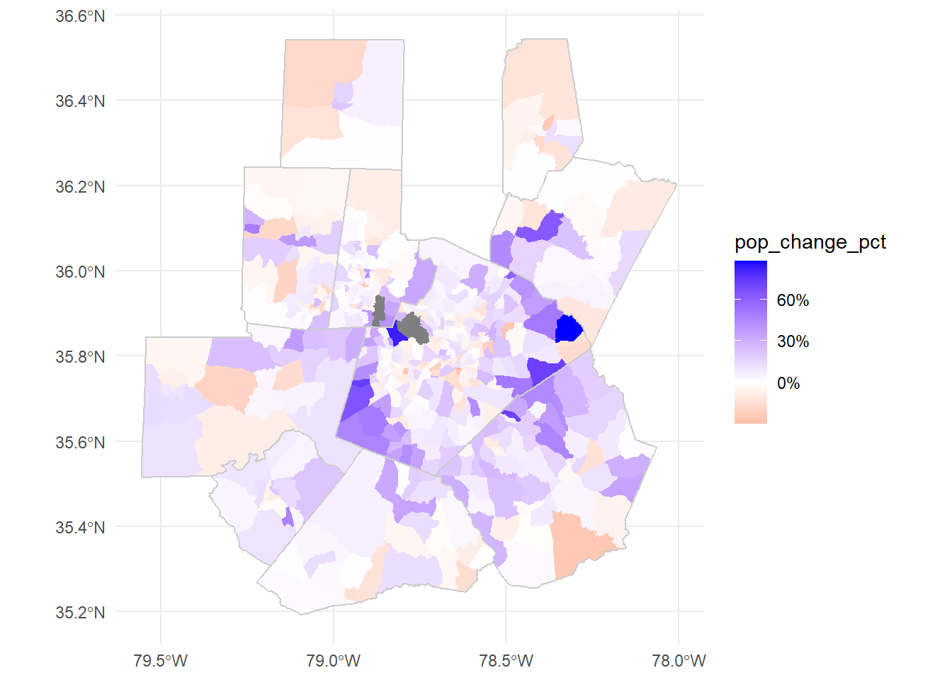

From non-spatial formats

Lots of spatial data doesn’t come in an explicitly spatial form. Let’s take a look at a CSV derived from Housing and Urban Development data (HUD).

Download nc_public_housing.csv

housing_raw <- read_csv('data/nc_public_housing.csv')

Rows: 228 Columns: 140
── Column specification ────────────────────────────────────────────────────────
Delimiter: ","
chr (37): PARTICIPANT_CODE, FORMAL_PARTICIPANT_NAME, DEVELOPMENT_CODE, PROJE...
dbl (98): X, Y, OBJECTID, TOTAL_UNITS, TOTAL_DWELLING_UNITS, ACC_UNITS, TOTA...
lgl  (5): PLACE_INC2KX, NECTA_NM, DPVRC, URB_OUT, ZIP_CLASS

ℹ Use `spec()` to retrieve the full column specification for this data.
ℹ Specify the column types or set `show_col_types = FALSE` to quiet this message.

head(housing_raw)

# A tibble: 6 × 140
      X     Y OBJECTID PARTICIPANT_CODE FORMAL_PARTICIPANT_NAME DEVELOPMENT_CODE
  <dbl> <dbl>    <dbl> <chr>            <chr>                   <chr>           
1 -80.0  35.9      151 NC006            Housing Authority of t… NC006000024     
2 -79.8  36.1      152 NC011            Housing Authority of t… NC011030095     
3 -80.2  36.1      153 NC012            Housing Authority of t… NC012000006     
4 -80.2  36.1      154 NC012            Housing Authority of t… NC012000030     
5 -78.0  35.4      155 NC015            Housing Authority of t… NC015000700     
6 -78.7  35.8      184 NC002            Housing Authority of t… NC002000015     
# ℹ 134 more variables: PROJECT_NAME <chr>, SCATTERED_SITE_IND <chr>,
#   PD_STATUS_TYPE_CODE <chr>, TOTAL_UNITS <dbl>, TOTAL_DWELLING_UNITS <dbl>,
#   ACC_UNITS <dbl>, TOTAL_OCCUPIED <dbl>, REGULAR_VACANT <dbl>,
#   PHA_TOTAL_UNITS <dbl>, PCT_OCCUPIED <dbl>, NUMBER_REPORTED <dbl>,
#   PCT_REPORTED <dbl>, MONTHS_SINCE_REPORT <dbl>, PCT_MOVEIN <dbl>,
#   PEOPLE_PER_UNIT <dbl>, PEOPLE_TOTAL <dbl>, RENT_PER_MONTH <dbl>,
#   SPENDING_PER_MONTH <dbl>, HH_INCOME <dbl>, PERSON_INCOME <dbl>, …

This dataset includes latitude and longitude data in two forms, X/Y and LAT/LON. Let’s check if they’re identical:

all(housing_raw$X==housing_raw$LON)

[1] TRUE

all(housing_raw$Y==housing_raw$LAT)

[1] TRUE

To use this as spatial data, we need to point out the spatial coordinates and define a coordinate reference system (CRS) with st_as_sf. With latitude and longitude data we can usually safely use WGS84 (ESPG: 4326). Even better, you may have documentation of the coordinate system used in the data.

housing <- st_as_sf(housing_raw, 
                    coords=c('X','Y'),
                    crs = 4326)

We can check or define the crs (not project into a new crs - this will not change your dataset or coordinates!) with st_crs. See ?st_crs1 for more information.

st_crs(housing)

Coordinate Reference System:
  User input: EPSG:4326 
  wkt:
GEOGCRS["WGS 84",
    ENSEMBLE["World Geodetic System 1984 ensemble",
        MEMBER["World Geodetic System 1984 (Transit)"],
        MEMBER["World Geodetic System 1984 (G730)"],
        MEMBER["World Geodetic System 1984 (G873)"],
        MEMBER["World Geodetic System 1984 (G1150)"],
        MEMBER["World Geodetic System 1984 (G1674)"],
        MEMBER["World Geodetic System 1984 (G1762)"],
        MEMBER["World Geodetic System 1984 (G2139)"],
        MEMBER["World Geodetic System 1984 (G2296)"],
        ELLIPSOID["WGS 84",6378137,298.257223563,
            LENGTHUNIT["metre",1]],
        ENSEMBLEACCURACY[2.0]],
    PRIMEM["Greenwich",0,
        ANGLEUNIT["degree",0.0174532925199433]],
    CS[ellipsoidal,2],
        AXIS["geodetic latitude (Lat)",north,
            ORDER[1],
            ANGLEUNIT["degree",0.0174532925199433]],
        AXIS["geodetic longitude (Lon)",east,
            ORDER[2],
            ANGLEUNIT["degree",0.0174532925199433]],
    USAGE[
        SCOPE["Horizontal component of 3D system."],
        AREA["World."],
        BBOX[-90,-180,90,180]],
    ID["EPSG",4326]]

There are a number of ways to get basemaps in R, but for today we’ll use the basemaps package. Maps from Carto are freely available without an API key. Most other services available through basemaps require a free sign up. st_bbox converts our set of points into a rectangle to form our plot area. We’ll use theme_nothing from ggmap to remove all axes and other plot elements.

#basemaps package map services use Web Mercator (ESPG: 3857)
basemap_ggplot(ext = st_bbox(housing), map_service = "carto")+
  geom_sf(data = housing)+
  coord_sf(crs = 3857)+ #ensures all layers are projected to match the basemap
  theme_nothing()

Warning: Transforming 'ext' to Web Mercator (EPSG: 3857), since 'ext' has a
different CRS. The CRS of the returned basemap will be Web Mercator, which is
the default CRS used by the supported tile services.

Loading basemap 'voyager' from map service 'carto'...

Coordinate system already present. Adding new coordinate system, which will
replace the existing one.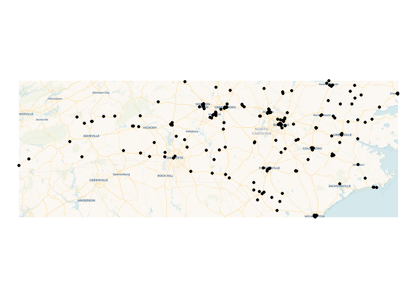

We can add a state boundary and some space using tigris and st_buffer.

nc_boundary <- states(progress_bar = FALSE) |> 
  filter(STUSPS=="NC") 

basemaps::basemap_ggplot(ext = st_bbox(st_buffer(nc_boundary, 
                                                 dist = 100000)), #distance in meters for geographic coordinates
                         map_service = "carto")+
  geom_sf(data = housing)+
  geom_sf(data = nc_boundary, fill=NA)+
  coord_sf(crs = 3857)+ #define the crs to match the boxplot
  ggmap::theme_nothing()

Warning: Transforming 'ext' to Web Mercator (EPSG: 3857), since 'ext' has a
different CRS. The CRS of the returned basemap will be Web Mercator, which is
the default CRS used by the supported tile services.

Loading basemap 'voyager' from map service 'carto'...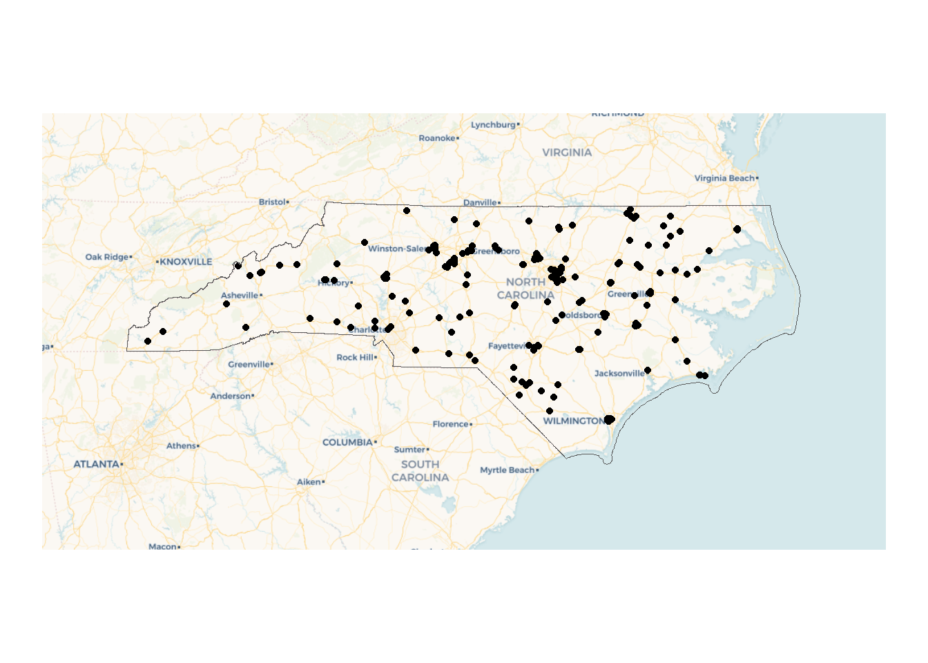

A note on coordinate systems

st_buffer is one of many spatial processing tools available in sf. Let’s plot the buffer, bounding box, and the state outline directly:

ggplot()+
  geom_sf(data = nc_boundary)+
  geom_sf(data = st_buffer(nc_boundary, dist = 50000), color = "blue", fill=NA)+
  geom_sf(data = st_as_sfc(st_bbox(st_buffer(nc_boundary, dist = 50000))), color = "red", fill = NA)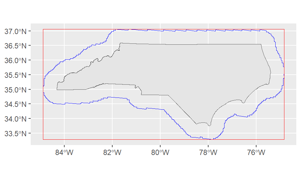

The jagged edges here are a result of working from a geographic or spherical coordinate system. They aren’t an issue for our use case since we’re just using this to quickly expand our bounding box.
However, if we were doing a more precise analysis this might be an issue! The solution is to convert our coordinates into a projected coordinate system (ESPG:31129 is a NAD83 state plane for North Carolina in meters) with st_transform. Since this coordinate system uses a plane instead of a sphere our buffers are smoother.

ggplot()+
  geom_sf(data = nc_boundary)+
  geom_sf(data = st_buffer(st_transform(nc_boundary, 32119), dist = 50000), color = "blue", fill=NA)+
  geom_sf(data = st_as_sfc(st_bbox(st_buffer(nc_boundary, dist = 50000))), color = "red", fill = NA)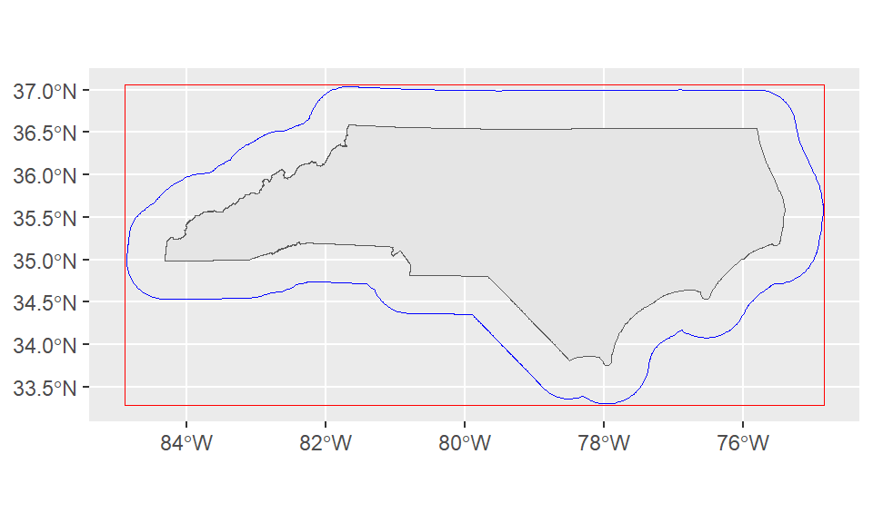

Loading data from ESRI data services

Let’s add state maintained roads to the map! We’ll use the ESRI data service from NC One Map. “NC DOT State Maintained Roads” is a Map Service that contains multiple layers.

To load data, we’ll need to specify a particular layer. On OneMap, you can click “I want to use this” > “View Data Source” to get to the MapServer directory page: https://gis11.services.ncdot.gov/arcgis/rest/services/NCDOT_StateMaintainedRoadsQtr/MapServer

This gives us most of what we’ll need to load the layer, but we still need to pick a layer under the “Layers” list. For today, let’s look at the simplest layer - Interstates (layer 2): https://gis11.services.ncdot.gov/arcgis/rest/services/NCDOT_StateMaintainedRoadsQtr/MapServer/2

The directory can be a nice way to explore what other data is available from a ESRI data service!

roads <- arc_read("https://gis11.services.ncdot.gov/arcgis/rest/services/NCDOT_StateMaintainedRoadsQtr/MapServer/2",
                  alias = "replace")

Registered S3 method overwritten by 'jsonify':
  method     from    
  print.json jsonlite

plot(st_geometry(roads))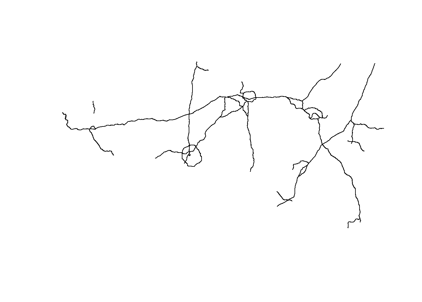

Let’s add it to our ggplot map! The order of our geoms is also the order in which they’re drawn, so we want to make sure our points are last and contextual layers like the nc boundary and roads come earlier in the code block.

Here we can add some more polish to the plot: - add colors for Urban vs Rural and label appropriately, update labels. - switch to the “light_no_labels” basemap from carto (see get_maptypes(map_service = "carto") for a full list of options). - add a scale and north arrow for context - various color and line tweaks for aesthetics

basemaps::basemap_ggplot(ext = st_bbox(st_buffer(nc_boundary, 
                                                 dist = 20000)), #distance in meters for geographic coordinates
                         map_service = "carto",
                         map_type = "light_no_labels")+
  geom_sf(data = nc_boundary, fill=NA, color = "grey70")+
  geom_sf(data = roads, color = "red", linewidth = 0.3)+
  geom_sf(data = housing,
          aes(color = UR), size = 2)+
  scale_color_brewer(palette = "Paired" ,labels = c("Rural", "Urban"), name = "Urban/Rural")+
  coord_sf(crs = 3857)+
  theme_minimal()+
  theme(legend.position="right")+
  annotation_scale(pad_x = unit(1.5, "cm"))+
  annotation_north_arrow(style=north_arrow_minimal)

Loading basemap 'light_no_labels' from map service 'carto'...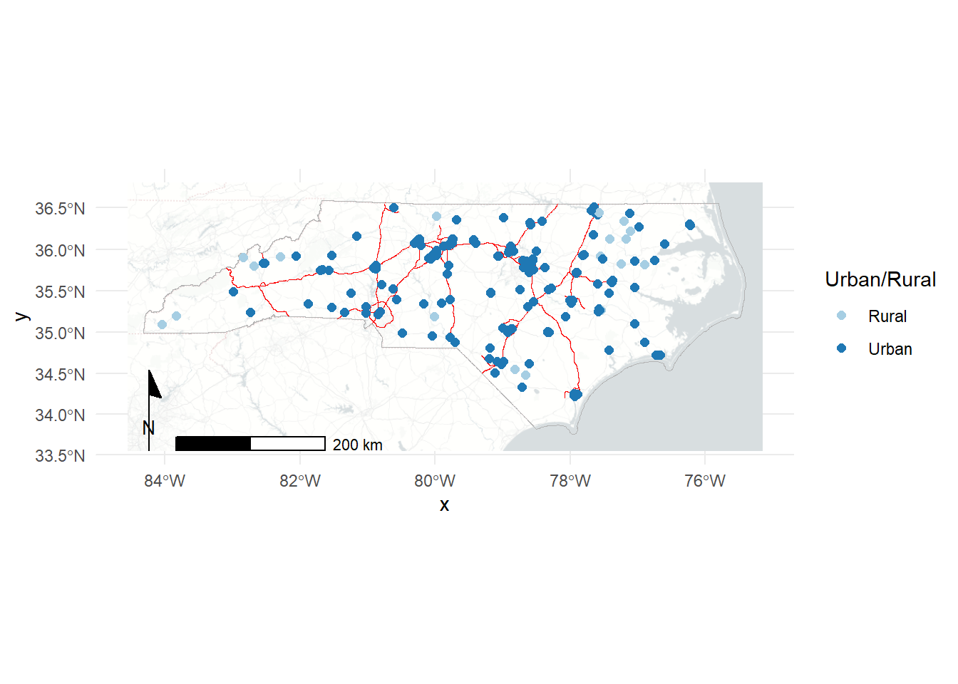

We could also forgo the basemap to make a simpler map:

ggplot()+
  geom_sf(data = nc_boundary, fill="grey90", color = "grey70")+
  geom_sf(data = roads, color = "red", stroke = 2)+
  geom_sf(data = housing,
          aes(color = UR), size=2)+
  theme_minimal()+
  scale_color_brewer(palette = "Paired" ,labels = c("Rural", "Urban"), name = "Urban/Rural")+
  coord_sf(crs = 3857)+
  theme(legend.position="right")+
  annotation_scale(pad_x = unit(1.5, "cm"))+
  annotation_north_arrow(style=ggspatial::north_arrow_minimal)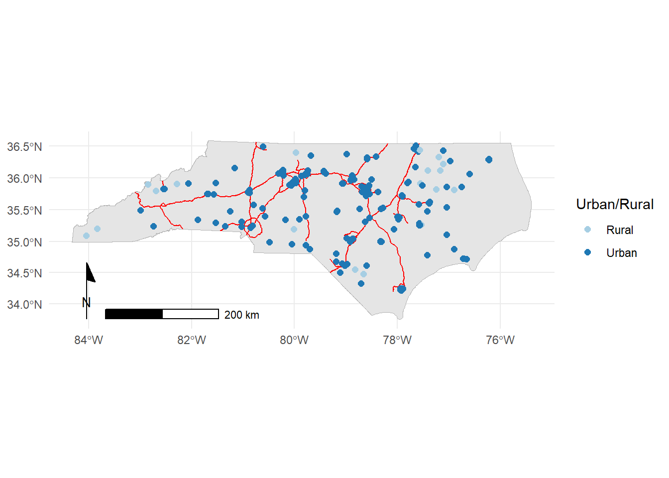

As usual, we could do much more to polish and fine tune these maps but this is a good start!

Basic spatial operations in R

We’ve already seen a simple spatial operation in st_buffer to create a buffered polygon expanding on an existing geometry. There are many other operations - we’ll focus on two major ideas: spatial filtering and spatial joins.

Spatial filters

Let’s use tigris to load polygons for all of the Combined Statistical Areas (CSAs) in the US.

us_csas <- combined_statistical_areas(progress_bar = FALSE)

We can use our housing dataset to pick out the CSAs that our housing projects touch. These won’t be purely in North Carolina since CSAs often cross state borders. We’ll use st_filter to spatially filter our CSAs to those related to the housing layer. The .predicate argument lets us define the relationship we’re looking for between the layers. ?st_intersects and DE-9IM provide more information about the relationships available. You can also define your own!

nc_csas <- us_csas |> 
  st_filter(housing, .predicate = st_intersects)

Error in `stopifnot()`:
ℹ In argument: `>...`.
Caused by error in `st_geos_binop()`:
! st_crs(x) == st_crs(y) is not TRUE

Uh oh! Unlike mapping which can often brush CRS issues under the rug, this fails because we haven’t made sure both our objects are in the same CRS. Let’s check.

st_crs(housing)

Coordinate Reference System:
  User input: EPSG:4326 
  wkt:
GEOGCRS["WGS 84",
    ENSEMBLE["World Geodetic System 1984 ensemble",
        MEMBER["World Geodetic System 1984 (Transit)"],
        MEMBER["World Geodetic System 1984 (G730)"],
        MEMBER["World Geodetic System 1984 (G873)"],
        MEMBER["World Geodetic System 1984 (G1150)"],
        MEMBER["World Geodetic System 1984 (G1674)"],
        MEMBER["World Geodetic System 1984 (G1762)"],
        MEMBER["World Geodetic System 1984 (G2139)"],
        MEMBER["World Geodetic System 1984 (G2296)"],
        ELLIPSOID["WGS 84",6378137,298.257223563,
            LENGTHUNIT["metre",1]],
        ENSEMBLEACCURACY[2.0]],
    PRIMEM["Greenwich",0,
        ANGLEUNIT["degree",0.0174532925199433]],
    CS[ellipsoidal,2],
        AXIS["geodetic latitude (Lat)",north,
            ORDER[1],
            ANGLEUNIT["degree",0.0174532925199433]],
        AXIS["geodetic longitude (Lon)",east,
            ORDER[2],
            ANGLEUNIT["degree",0.0174532925199433]],
    USAGE[
        SCOPE["Horizontal component of 3D system."],
        AREA["World."],
        BBOX[-90,-180,90,180]],
    ID["EPSG",4326]]

st_crs(us_csas)

Coordinate Reference System:
  User input: NAD83 
  wkt:
GEOGCRS["NAD83",
    DATUM["North American Datum 1983",
        ELLIPSOID["GRS 1980",6378137,298.257222101,
            LENGTHUNIT["metre",1]]],
    PRIMEM["Greenwich",0,
        ANGLEUNIT["degree",0.0174532925199433]],
    CS[ellipsoidal,2],
        AXIS["latitude",north,
            ORDER[1],
            ANGLEUNIT["degree",0.0174532925199433]],
        AXIS["longitude",east,
            ORDER[2],
            ANGLEUNIT["degree",0.0174532925199433]],
    ID["EPSG",4269]]

Let’s go with NAD83 for now, since that’s the default for census data. We can use st_transform to move

housing_nad <- st_transform(housing, crs = 4269)
# #or alternatively:
# housing_nad <- st_transform(housing, crs = st_crs(us_csas))

nc_csas <- us_csas |> 
  st_filter(housing_nad, .predicate = st_intersects)

Note that we filter with the housing locations not the NC boundary. There are several CSAs that touch NC and would be captured if we used that as a filter:

nc_csas_border <- us_csas |> 
  st_filter(nc_boundary, .predicate = st_intersects)
nrow(nc_csas)

[1] 9

nrow(nc_csas_border)

[1] 14

However, we could work around this by using the centroids of the CSAs with st_centroid.

nc_csas_centroids <- st_centroid(us_csas) |> 
  st_filter(nc_boundary, .predicate = st_intersects)

Warning: st_centroid assumes attributes are constant over geometries

nrow(nc_csas_centroids)

[1] 9

The only downside is this leaves us with centroid geometries instead of polygons.

ggplot()+
  geom_sf(data = nc_csas_border, fill = "red", alpha = 0.5, color=NA)+
  geom_sf(data=nc_csas, color=NA)+
  geom_sf(data=nc_csas_centroids)+
  geom_sf(data = nc_boundary, fill=NA)+
  theme_minimal()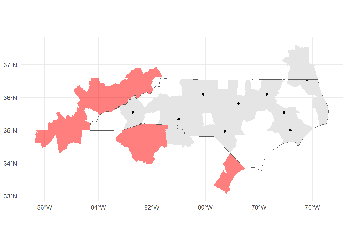

We’ll work with our original nc_csas. Now that we’ve limited our CSAs, let’s take a look at what made the cut.

ggplot()+
  geom_sf(data = nc_csas, aes(fill = NAME))+
  geom_sf(data = nc_boundary, fill = NA, linetype = "dashed")+
  theme_minimal()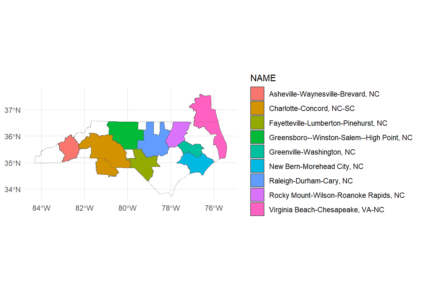

Spatial joins

Another very useful spatial operation is the spatial join (st_join). This uses a similar predicate to the spatial filter to determine the relationship to join on. st_intersects is again the default.

After joining, we drop geometries to do some dplyr transformations to calculate the number of developments, number of housing units, and average percent occupied in each CSA. Dropping geometries speeds up the calculation by simplifying the dataset. Then we rejoin to the spatial data as a last step!

csa_housing <- st_join(nc_csas, housing_nad, join = st_intersects) |> 
  st_drop_geometry() |>
  group_by(CSAFP) |> 
  summarize(ct = n(),
            units = sum(PHA_TOTAL_UNITS, na.rm=T),
            avg_pct_occ = mean(PCT_OCCUPIED, na.rm=T)) |> 
  right_join(nc_csas, y = _)

Joining with `by = join_by(CSAFP)`

Finally, we can plot our newly calculated values!

ggplot()+
  geom_sf(data = csa_housing, aes(fill = avg_pct_occ))+
  geom_sf(data = nc_boundary, fill = NA, linetype = "dashed")+
  geom_sf(data = housing_nad, size = 0.5)+
  scale_fill_gradient(low = "white", high = "darkred")+
  theme_minimal()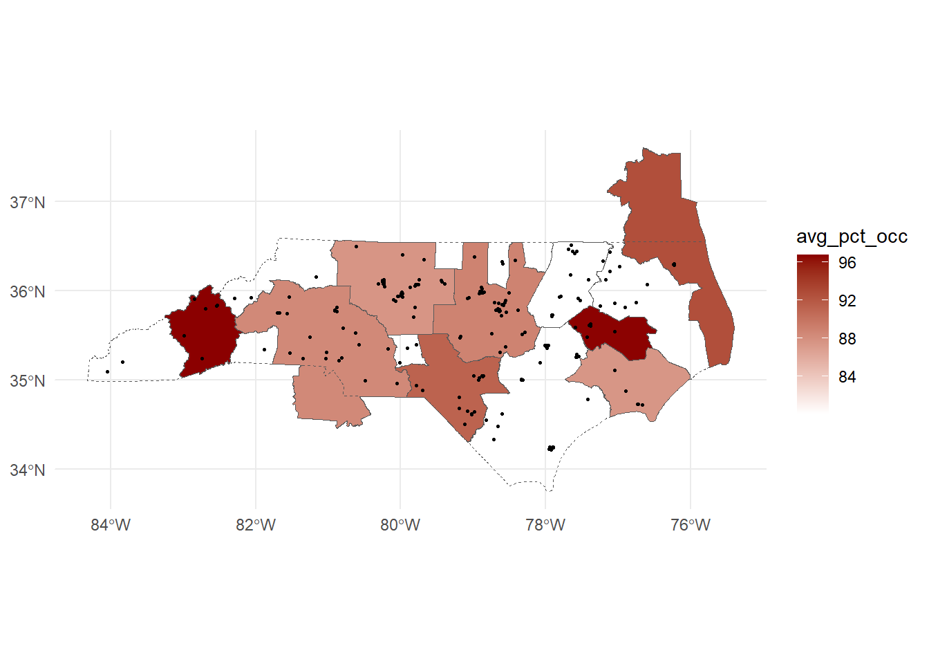

In practice, these types of calculations may also feed into tables, graphs and other statistical analyses!

Other mapping packages

tmap

tmap is another popular package for making thematic maps.

library(tmap)
tm_basemap("CartoDB.Positron")+
  tm_shape(nc_csas)+
  tm_polygons(fill="NAME", fill_alpha = 0.5,
              fill.legend = tm_legend(
                position = tm_pos_out("right", "center", pos.h = "center")
              ))+
  tm_shape(housing)+
  tm_dots()+
  tm_compass()+
  tm_scalebar()+
  tm_layout(frame = FALSE, 
            inner.margins = c(0.1,0.1,0,0)) #add space inside the plot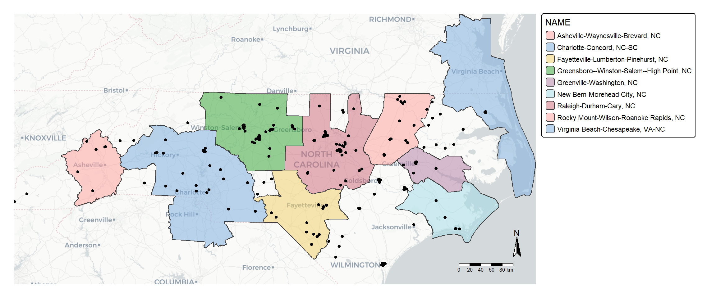

By adding tmap_mode("view") before our code, we can make an interactive map.

tmap_mode("view")

ℹ tmap modes "plot" - "view"
ℹ toggle with `tmap::ttm()`

tm_basemap("CartoDB.Positron")+
  tm_shape(nc_csas)+
  tm_polygons(fill="NAME", fill_alpha = 0.5,
              fill.legend = tm_legend(
                position = tm_pos_out("right", "center", pos.h = "center")
              ))+
  tm_legend_hide()+
  tm_shape(housing)+
  tm_dots()+
  tm_compass()+
  tm_scalebar()+
  tm_layout(frame = FALSE, 
            inner.margins = c(0.1,0.1,0,0)) #add space inside the plot

── tmap v3 code detected ───────────────────────────────────────────────────────
[v3->v4] `tm_legend()`: use 'tm_legend()' inside a layer function, e.g.
'tm_polygons(..., fill.legend = tm_legend())'

Leaflet

leaflet is the R package for creating interactive maps with the Leaflet JavaScript library.

Other data formats

Raster data

There are two major raster packages to know about! terra is the successor to the raster package and works well for most simple rasters. stars is a better fit for cubes of data - think rasters with many many layers covering lots of different time points. stars itself is short for “Spatiotemporal Arrays”!

Shapefiles and geopackages

Shapefiles are an older format with some significant limitations (like variable name lengths!), but they’re important to be familiar with because they’re very very common and quirky. Despite the name, a shapefile is actually a collection of files that have to be stored together - anywhere from 3 to 12 files! It’s good practice to share them as a zipped folder.

Geopackages are a newer file format that avoid many of the limitations of shapefiles.

There are lots of other spatial formats out there like KML, GeoJSON, PostGIS and many more! R can work with many of these but we won’t work with them all today.

File geodatabases

File Geodatabases (.gdb) is a folder-based format that can store and manage multiple spatial and non-spatial data sets. It is a common data type if you work frequently in ArcGIS Pro and a proprietary format from Esri. Spatial layers can be read in as sf objects using st_read and specifying the geodatabase and layer names: st_read(dsn, layer)

You can also write a new or modified layer to a file geodatabase using st_write. Here is an example:

st_write(obj = nc_boundary, 
         dsn = "nc_project.gdb", 
         layer = "nc",
         driver = "OpenFileGDB",
         delete_dsn = FALSE,
         delete_layer = TRUE)

Where dsn is the path to your geodatabase, layer is the name you like to give the object in the file geodatabase, and delete_dsn specifies if you would like to delete the file geodatabse and create a new one. Typically, you will get an error if a layer of the same name already exists, but delete_layer = TRUE will overwrite the existing feature class.

“OpenFileGDB” is the built-in driver that works with Esri File Geodatabases. You can also leave out the driver argument; a driver name is typically accurately guessed and allows the object to write.

Learn more: CRAN Task View

To learn more about other R packages around spatial data processing and analysis, consult the CRAN Task View: Analysis of Spatial Data.

For example, the spdep and spatialreg packages provide functions for weights-matrix based methods like Moran’s I and Spatial Autoregressive Models.