beginR: Workflows and Objects

Author

University of North Carolina at Chapel Hill

Data and other downloads

Airbnb listings from Washington DC

Today

This introductory workshop aims to cover:

Reproducible workflow
- importing data
- scripts
- projects
- saving output
R for Data Science Chapters 4,6,8

What is reproducibility?

Scientific reproducibility - if you repeat my experiment, you will get the same results as me. This is beyond the scope of this workshop (see here for an overview)
Computational reproducibility - if I give you my data and code, you will get the same results as me. We’ll focus on the basics of computational reproducibility today.

Why does computational reproducibility matter?

Your most important collaborator is you six months from now.
We want Science (with a capital S) to be self-correcting. Since you’re human, you will make mistakes, so you want to make it as easy as possible for others to catch your errors (see the Reinhart and Rogoff Excel error and the Guinea worm wars for recent examples)

Your script is real, your environment is not

For your results to be reproducible, every step you take to manipulate the data should be explicitly documented in an R script.

This also means that you want to make sure that your results don’t have hidden/implicit dependencies in your R environment. There are two steps you can to take to prevent this.

Reconfigure RStudio not to save your workspace between sessions. (Tools > Global Options > General)
Restart RStudio from scratch and rerun the current script often.
- Cmd/Ctrl + Shift + F10 to restart RStudio
- Cmd/Ctrl + Shift + S to rerun the current script

Note: If you have learned R in the past, you may have been taught to use the expression rm(list = ls()) to clear your R environment. This will not actually return R to a blank slate! Although this code will delete objects in your R environment, it won’t reset global settings that have been changed. It is always safer and more effective to restart RStudio.

1: RStudio Projects

You can use the R function setwd() to point to locations of data files, but this isn’t ideal for reproducible research. When you switch between computers, it is likely that the absolute directory path will change, so you will have to modify the path for each computer. Users of your code will not have the same absolute directory path that you have, so they will have to modify the path in the setwd() function before they can use your code.

RStudio Projects provide a way to bundle together data, code, and other files together so that you can refer to files with relative directory paths, which creates a much more portable structure that won’t need to be modified between computers or users.

Configuration

File > New Project > New Directory > New Project
Create a new subdirectory called “data” inside this project to store the data.
Copy the Airbnb data (listings.csv) into this data directory
Create a new R Script for the data analysis in this project. (File > New File > R Script)

2: Import the data

We’ll begin by loading the tidyverse library. This library includes readr, which we will use to read in our data file (for more details on readr, see Chapter 11 of the text).

RStudio has a useful keyboard shortcut for <- (the assignment operator): Alt + -, i.e. press the Alt key and the minus/hyphen key at the same time.

# Purpose: Exploratory data analysis of airbnb data
# Author: Nuvan Rathnayaka
# Date: September 2018

# Setup -----------------------------------------------------------
library(tidyverse)

── Attaching core tidyverse packages ──────────────────────── tidyverse 2.0.0 ──
✔ dplyr     1.1.4     ✔ readr     2.1.4
✔ forcats   1.0.0     ✔ stringr   1.5.1
✔ ggplot2   3.5.0     ✔ tibble    3.2.1
✔ lubridate 1.9.3     ✔ tidyr     1.3.1
✔ purrr     1.0.2     
── Conflicts ────────────────────────────────────────── tidyverse_conflicts() ──
✖ dplyr::filter() masks stats::filter()
✖ dplyr::lag()    masks stats::lag()
ℹ Use the conflicted package (<http://conflicted.r-lib.org/>) to force all conflicts to become errors

# Data Import ------------------------------------------------------
airbnb_dc <- read_csv("data/listings.csv") #Since I'm using an RStudio project, I only have to specify the path relative to the top directory

Rows: 7788 Columns: 14
── Column specification ────────────────────────────────────────────────────────
Delimiter: ","
chr  (4): name, property_type, room_type, cancellation_policy
dbl (10): id, accommodates, bathrooms, bedrooms, price, extra_people, minimu...

ℹ Use `spec()` to retrieve the full column specification for this data.
ℹ Specify the column types or set `show_col_types = FALSE` to quiet this message.

#If you have problems running the read_csv above, the following code should also work
#(Download data directly from the internet)
#airbnb_dc <- read_csv(url("https://unc-libraries-data.github.io/R-Open-Labs/week2_Workflow/data/listings.csv"))

Reminder: Comments

In R, the # symbol indicates the beginning of a comment. Everything to the right of that is ignored by R, so you can write plain text to document what you’re doing, organize your code, and explain any tricky or unusual steps.

Coding conventions

Something that I’ve glossed over is that you have options for how to name objects. For example, we called our imported data airbnb_dc, but we could have called it airbnbListings, or airbnb.listings

Having a consistent way you name objects and functions helps you remember what things are called. It’s especially useful when you’re working with others to agree upon a coding convention. It doesn’t particularly matter which one you choose, as long as you choose a convention and stick to it.

Example style guide: http://style.tidyverse.org/index.html

3: Objects and classes

R is an object-oriented programming language. One way to understand how objects work in programming is to look at how objects work in real life.

We tend to group objects by their structure. For example, there are many objects we call cars, and they all tend to share similarities in structure - they have wheels, windows, doors, etc. An individual car such as my car or your car is an instance of this structure. Cars also have a set of properties such as make, model, year and color. Each individual car has some variation of these properties.

Objects in R work in a similar way.

In the diagram above, we are looking at three common data structures often used in R: vectors, matrices and data frames. We can create individual objects from these data structures, and those objects have their own properties. The way R defines what properties a given object has is through it’s class. You can think of a class as a contract between R and its users, defining the structure and properties of an object. People who develop R libraries take advantage of this system to reliably customize the behavior of functions.

Vectors

Vectors are the most basic collection of items, often created with c(). Depending on what you put into a vector, it also automatically decides a type. The most common types are: numeric (integer or double), character, and logical.

c(1,2,3,4) #Numeric (integer)

[1] 1 2 3 4

c(1.4,2.7,3.2) #Numeric (double)

[1] 1.4 2.7 3.2

c("cat","dog","fish") #Character

[1] "cat"  "dog"  "fish"

c(TRUE,FALSE,TRUE) #Logical

[1]  TRUE FALSE  TRUE

c("cat",1,FALSE) #Character - check other combinations yourself!

[1] "cat"   "1"     "FALSE"

Vectors only have one dimension: length (accessible with the length function.)

We’ll learn more about another special case of vectors, “factors”, as the semester goes on.

Matrices

Matrices are two-dimensional generalizations of vectors. The dimensions of a matrix are the number of rows and the number of columns (in that order).

Like vectors, matrices have a single type, and we’ll most commonly see numeric, character, and logical types.

matrix(1:9,nrow=3,ncol=3)

     [,1] [,2] [,3]
[1,]    1    4    7
[2,]    2    5    8
[3,]    3    6    9

#1:9 is equivalent to c(1,2,3,4,5,6,7,8,9)

Data.frames

Like a matrix, the data.frame has rows and columns, but each column can have its own different data type. This is the most common way to store datasets in R.

For example, our airbnb_dc dataset has been read into a data.frame. We can check its type with class.

class(airbnb_dc)

[1] "spec_tbl_df" "tbl_df"      "tbl"         "data.frame"

We can see that airbnb_dc has multiple classes! "tbl_df" and "tbl" indicate that this data.frame is also a “tibble”.

One way to extract a single column from a dataframe uses the $ operator with the column’s name.

class(airbnb_dc$property_type)

[1] "character"

Useful data.frame commands

The dim() function will print the dimensions (rows x columns) of your data frame.

head() will print the first few rows of your data frame. glimpse() transposes the data.frame for easier printing of similar output.

(Note: str() is a general purpose function similar to glimpse that will display the structure of an object, often including extra information. This can be useful for debugging.)

# Some useful functions  ----------------------------------------
dim(airbnb_dc)

[1] 7788   14

head(airbnb_dc)

# A tibble: 6 × 14
        id name    property_type room_type accommodates bathrooms bedrooms price
     <dbl> <chr>   <chr>         <chr>            <dbl>     <dbl>    <dbl> <dbl>
1  4873463 Cozy P… Apartment     Entire h…            3       1          0    95
2 16736650 Large,… Apartment     Entire h…            2       1          0   200
3 14999877 Newly … Apartment     Entire h…            2       1          1   100
4  5955860 Spacio… Apartment     Entire h…            3       1          1   129
5 15655208 Luxury… Townhouse     Entire h…            4       2.5        2   500
6  4022565 Dupont… Apartment     Private …            2       2.5        1   110
# ℹ 6 more variables: extra_people <dbl>, minimum_nights <dbl>,
#   number_of_reviews <dbl>, review_scores_rating <dbl>,
#   cancellation_policy <chr>, reviews_per_month <dbl>

glimpse(airbnb_dc)

Rows: 7,788
Columns: 14
$ id                   <dbl> 4873463, 16736650, 14999877, 5955860, 15655208, 4…
$ name                 <chr> "Cozy Pied-a-Terre, the Heart of DC", "Large, wel…
$ property_type        <chr> "Apartment", "Apartment", "Apartment", "Apartment…
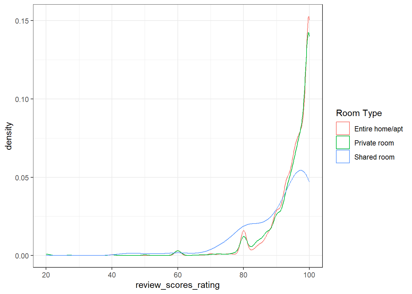
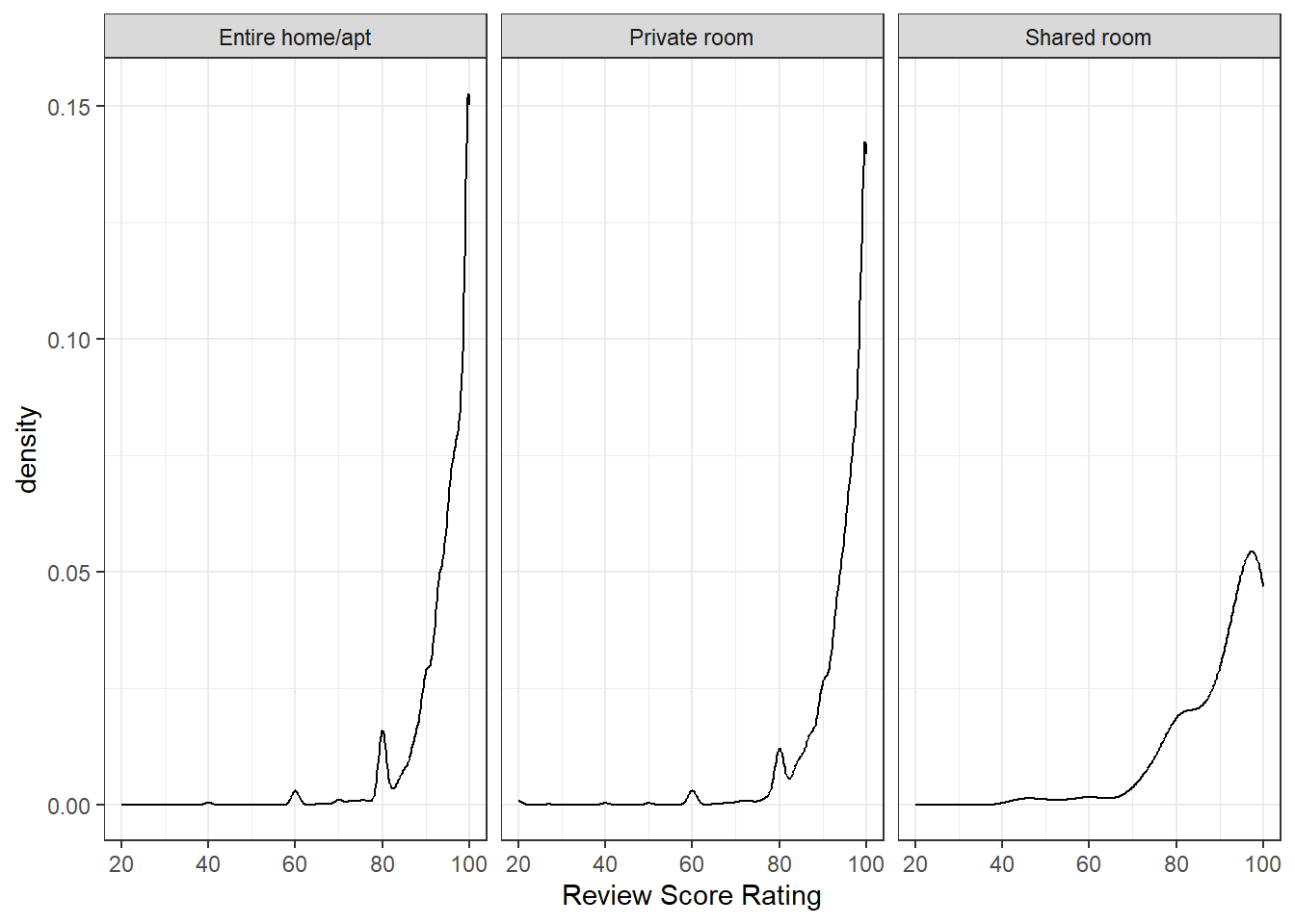
$ room_type            <chr> "Entire home/apt", "Entire home/apt", "Entire hom…
$ accommodates         <dbl> 3, 2, 2, 3, 4, 2, 3, 2, 4, 2, 4, 3, 2, 2, 2, 2, 2…
$ bathrooms            <dbl> 1.0, 1.0, 1.0, 1.0, 2.5, 2.5, 1.0, 1.0, 1.0, 1.0,…
$ bedrooms             <dbl> 0, 0, 1, 1, 2, 1, 1, 1, 2, 1, 2, 1, 0, 0, 1, 0, 1…
$ price                <dbl> 95, 200, 100, 129, 500, 110, 225, 79, 172, 110, 1…
$ extra_people         <dbl> 10, 0, 0, 50, 0, 15, 20, 0, 0, 10, 0, 0, 0, 0, 20…
$ minimum_nights       <dbl> 2, 1, 27, 2, 2, 6, 3, 3, 1, 1, 2, 1, 2, 3, 7, 2, …
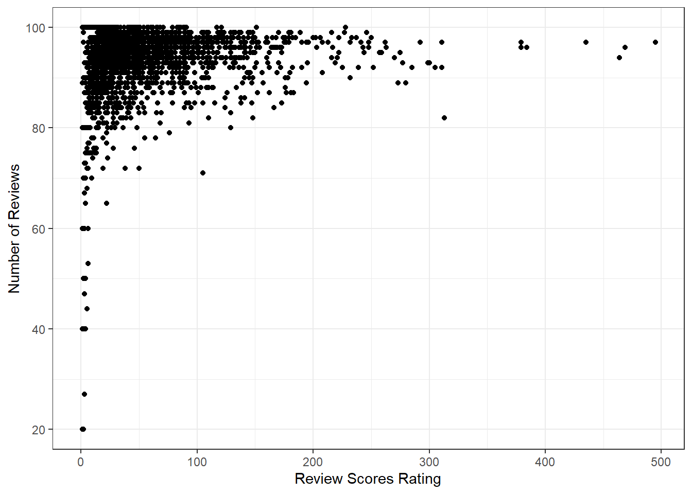
$ number_of_reviews    <dbl> 29, 2, 0, 79, 1, 7, 3, 4, 24, 4, 0, 0, 23, 3, 6, …
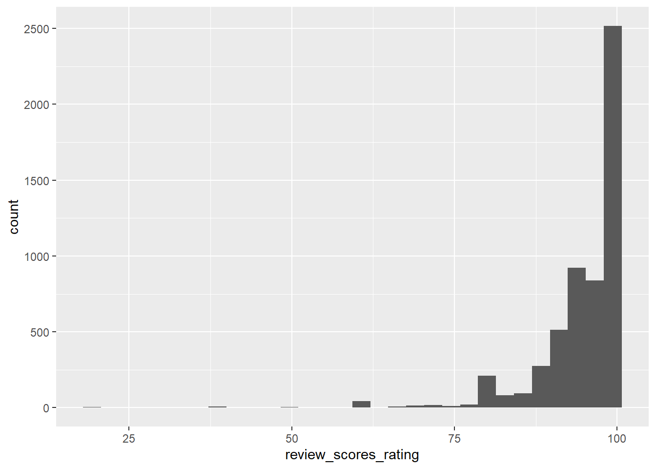
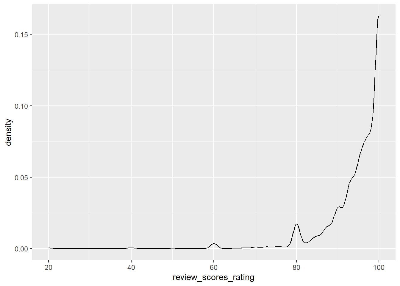
$ review_scores_rating <dbl> 94, 90, NA, 85, 100, 97, 100, 89, 88, 100, NA, NA…
$ cancellation_policy  <chr> "flexible", "flexible", "moderate", "flexible", "…
$ reviews_per_month    <dbl> 1.01, 0.55, NA, 3.13, 1.00, 0.23, 0.82, 0.09, 0.4…

4: Tables for categorical data

We can use the table() function to view counts/frequencies of categorical variables.

# Categorical Variables  ----------------------------------------
table(airbnb_dc$property_type)


         Apartment    Bed & Breakfast               Boat     Boutique hotel 
              4191                 73                  3                 11 
          Bungalow              Cabin             Castle        Condominium 
                 4                  1                  1                420 
              Dorm        Guest suite         Guesthouse             Hostel 
                25                 11                 17                  2 
             House             In-law               Loft              Other 
              2480                 12                 33                 31 
Serviced apartment          Timeshare          Townhouse              Train 
                 1                  1                468                  1 
         Treehouse              Villa 
                 1                  1

As we saw in week 1, you can also next functions within each other. Here, let’s generate a contingency table using table(), then sort it by count using sort().

sort(table(airbnb_dc$property_type), decreasing=TRUE)


         Apartment              House          Townhouse        Condominium 
              4191               2480                468                420 
   Bed & Breakfast               Loft              Other               Dorm 
                73                 33                 31                 25 
        Guesthouse             In-law     Boutique hotel        Guest suite 
                17                 12                 11                 11 
          Bungalow               Boat             Hostel              Cabin 
                 4                  3                  2                  1 
            Castle Serviced apartment          Timeshare              Train 
                 1                  1                  1                  1 
         Treehouse              Villa 
                 1                  1

That works, but it’s a little hard to read. We could try breaking this into two steps and storing our intermediate output.

property_type_table <- table(airbnb_dc$property_type)
sort(property_type_table, decreasing = TRUE)


         Apartment              House          Townhouse        Condominium 
              4191               2480                468                420 
   Bed & Breakfast               Loft              Other               Dorm 
                73                 33                 31                 25 
        Guesthouse             In-law     Boutique hotel        Guest suite 
                17                 12                 11                 11 
          Bungalow               Boat             Hostel              Cabin 
                 4                  3                  2                  1 
            Castle Serviced apartment          Timeshare              Train 
                 1                  1                  1                  1 
         Treehouse              Villa 
                 1                  1

This works ok, but it does mean we’re creating an additional object, property_type_table, and we could end up with lots of objects that are trivially different from each other if we do this too often. In the next lesson, we’ll introduce the pipe operator, which makes this kind of nested computation easier to read.

Suppose we want to know whether a listings price is greater than 500. We can create a logical type vector as follows (output suppressed for space):

airbnb_dc$price > 500 #Note that since we're not assigning this vector to a variable, R displays it, but doesn't save it as an object in the environment.

You can see other logical operators here.

We can feed this logical vector into the table() function to get a count of how many listings have prices above $500.

table(airbnb_dc$price > 500)


FALSE  TRUE 
 7029   759

We can also use the table function to look at the joint counts of multiple categorical variables. For example, if we want to look at the how many properties have prices above $500 across different property types.

with(airbnb_dc, table(property_type, price > 500))

                    
property_type        FALSE TRUE
  Apartment           3884  307
  Bed & Breakfast       72    1
  Boat                   3    0
  Boutique hotel        11    0
  Bungalow               4    0
  Cabin                  1    0
  Castle                 1    0
  Condominium          356   64
  Dorm                  25    0
  Guest suite           11    0
  Guesthouse            16    1
  Hostel                 2    0
  House               2150  330
  In-law                12    0
  Loft                  28    5
  Other                 28    3
  Serviced apartment     1    0
  Timeshare              1    0
  Townhouse            420   48
  Train                  1    0
  Treehouse              1    0
  Villa                  1    0

5: Exploring continuous data

R has built-in functions to compute the mean, standard deviation, min, median, and max.

# Continuous Variables  ----------------------------------------

mean(airbnb_dc$price)

[1] 247.1451

sd(airbnb_dc$price)

[1] 385.8856

min(airbnb_dc$price)

[1] 0

median(airbnb_dc$price)

[1] 125

max(airbnb_dc$price)

[1] 6000

R also has a built-in function to compute correlation coefficients. This let’s us explore the pairwise associations between continuous variables.

with(airbnb_dc, cor(price, number_of_reviews))

[1] -0.1560021

6: Missing data

There are some missing values in the review_scores_rating and reviews_per_month columns, even within the first six rows. We can check which values of review_scores_rating are NA with is.na()

# Continuous Variables  ----------------------------------------


sum(is.na(airbnb_dc$review_scores_rating)) #summing a logical (TRUE/FALSE) vector counts the number of TRUE values

[1] 2207

We can check all of our columns using R’s colSums to sum all of the columns at the same time.

colSums(is.na(airbnb_dc))

                  id                 name        property_type 
                   0                    5                    0 
           room_type         accommodates            bathrooms 
                   0                    0                   14 
            bedrooms                price         extra_people 
                  14                    0                    0 
      minimum_nights    number_of_reviews review_scores_rating 
                   0                    0                 2207 
 cancellation_policy    reviews_per_month 
                   0                 2128

Handling missing data is an advanced topic that is a bit beyond the scope of this lesson. There is no good way to handle missing data, there are only bad and less bad ways.

One of the bad ways to handle missing data is what’s known as a complete case analysis. In this kind of analysis, you only keep observations (rows) where you have observed (non-missing) values for ALL columns.

R has built-in functions to facilitate this:

complete.cases returns a logical vector indicating whether or not an entire row of a dataset contains any missing values. You can also use this function on a subset of columns to determine if only those columns are complete
na.omit returns a new dataframe with only the complete cases (as identified above)

For most R functions, the default is to return NA is any of the values are NA:

mean(airbnb_dc$review_scores_rating)

[1] NA

with(airbnb_dc, cor(review_scores_rating, reviews_per_month))

[1] NA

Some functions, like the linear regression function lm(), perform a complete-case analysis automatically:

lm(review_scores_rating~price, data=airbnb_dc)


Call:
lm(formula = review_scores_rating ~ price, data = airbnb_dc)

Coefficients:
(Intercept)        price  
  94.230536     0.003191

When a function complains about missing values and fails, there’s usually an argument that can be modified to change it to a complete-case analysis:

mean(airbnb_dc$review_scores_rating, na.rm=TRUE)

[1] 94.72406

with(airbnb_dc, cor(review_scores_rating, reviews_per_month, use="pairwise.complete.obs"))

[1] 0.09933035

7: Saving output

Suppose, we’ve done some computation, and we want to save our modified dataframe. We can use write_csv() to save our dataset as comma separated values file.

airbnb_dc$price_gt_500 <- (airbnb_dc$price > 500)
write_csv(airbnb_dc, "data/modified_airbnb.csv")

8: ggplot (time allowing)

Last week, we introduced ggplot2 for statistical graphics. This library implements the grammar of graphics, which provides a structured, modular way to think about plots. The three most commonly altered components are:

aesthetics - the visual properties of objects on the plot, e.g x location, y location, color, size
geom - the geometric object used to represent your data, e.g. point, line, histogram
facets - let you create subplots for each level of a categorical variable

Let’s look at a few examples. We can look at a histogram of review scores. Here, the only aesthetic we need to set is the x location, and then we can request a histogram.

ggplot(airbnb_dc, aes(x=review_scores_rating)) + geom_histogram()

`stat_bin()` using `bins = 30`. Pick better value with `binwidth`.

Warning: Removed 2207 rows containing non-finite outside the scale range
(`stat_bin()`).

To get a smoothed histogram (aka kernel density estimate), all we have to do is change to geom_density:

ggplot(airbnb_dc, aes(x=review_scores_rating)) + geom_density()

Warning: Removed 2207 rows containing non-finite outside the scale range
(`stat_density()`).

If we want to look at the distribution of reviews across different room types, we could add a group aesthetic for the room_type variable:

ggplot(airbnb_dc, aes(x=review_scores_rating, color=room_type)) + geom_density() + guides(color=guide_legend(title="Room Type")) + theme_bw()

Warning: Removed 2207 rows containing non-finite outside the scale range
(`stat_density()`).

Since, there a lot of overlap, we could use facets to create a subplot for each room_type:

ggplot(airbnb_dc, aes(x=review_scores_rating, color=)) + geom_density() + facet_wrap(~ room_type) + xlab("Review Score Rating") + theme_bw()

Warning: Removed 2207 rows containing non-finite outside the scale range
(`stat_density()`).

So far, we’ve looked a single continuous variable (review_scores_rating) as it related to a categorical variables (room_type). If we want to look at how two continuous variables are related, we could create a scatterplot by specifiying x and y aesthetics and using geom_point()

ggplot(data=airbnb_dc,aes(x=number_of_reviews,y=review_scores_rating))+
  geom_point() + xlab("Review Scores Rating") + ylab("Number of Reviews") + theme_bw()

Warning: Removed 2207 rows containing missing values or values outside the scale range
(`geom_point()`).

Again, we can use facets to look at how this varies across room_type:

ggplot(data=airbnb_dc,aes(x=number_of_reviews,y=review_scores_rating))+
  geom_point() + xlab("Review Scores Rating") + ylab("Number of Reviews") + theme_bw() + facet_wrap(~ room_type)

Warning: Removed 2207 rows containing missing values or values outside the scale range
(`geom_point()`).

Additional resources

Why setwd() is bad practice

Concise guide to basic computational reproducibility

Eight things you can do to make your open science more understandable

A detailed guide to reproducible workflows in collaborative settings

Exercises

What are the different types of cancellation policies offered at Airbnb?
What is the most common and least common cancellation policy?
What percent of Airbnb property types are houses? Hint: To find what percent of X is Y, use this formula: Y/X * 100
How many listings get a review rating below 50?
Try generating a scatterplot of price against bedrooms. Now add an overlay of a loess line. Now try creating subplots for each of the property types.
Try installing the visdat library, and explore different ways to visualize missing data.