#install.packages("naniar")
library(naniar)
#install.packages("Hmisc")
library(Hmisc)Extra - Missing Data Tools
Necessary Packages
Missing data is an advanced topic, and this document does not provide a comprehensive treatment of how to handle missing data in statistical modeling. These are just two tools that I’m fond of. For this document, I’ll be using the built-in airquality dataset. Before you proceed, make sure to install the naniar and Hmisc R packages.
Missing data visualization
The naniar package provides lots of tools for understanding the nature of the missingness.
data("airquality")
vis_miss(airquality)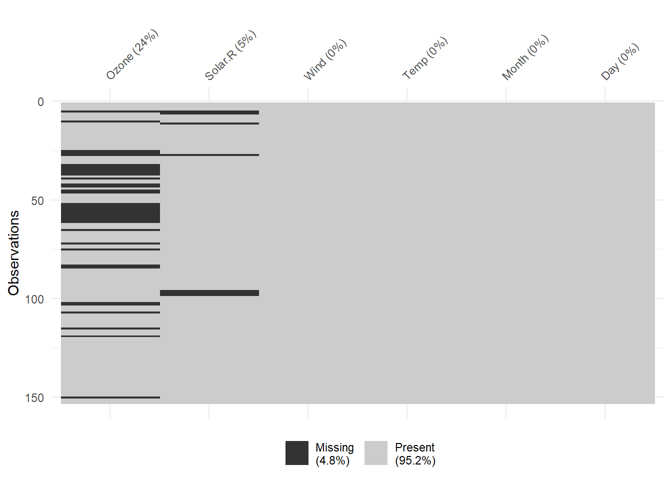
naniar also includes the upset plot to explore the patterns of missingness. We can clearly see there are only two observations that are missing both Ozone and Solar.R.
gg_miss_upset(airquality)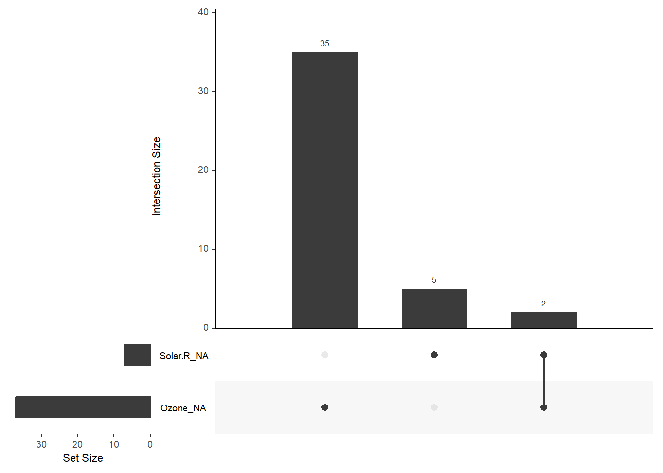
It also introduces a new geom that extends the capabilities of ggplot. By default, ggplot removes rows with missing values.
ggplot(airquality,
       aes(x = Ozone,
           y = Solar.R)) +
  geom_point()
Warning: Removed 42 rows containing missing values or values outside the scale range
(`geom_point()`).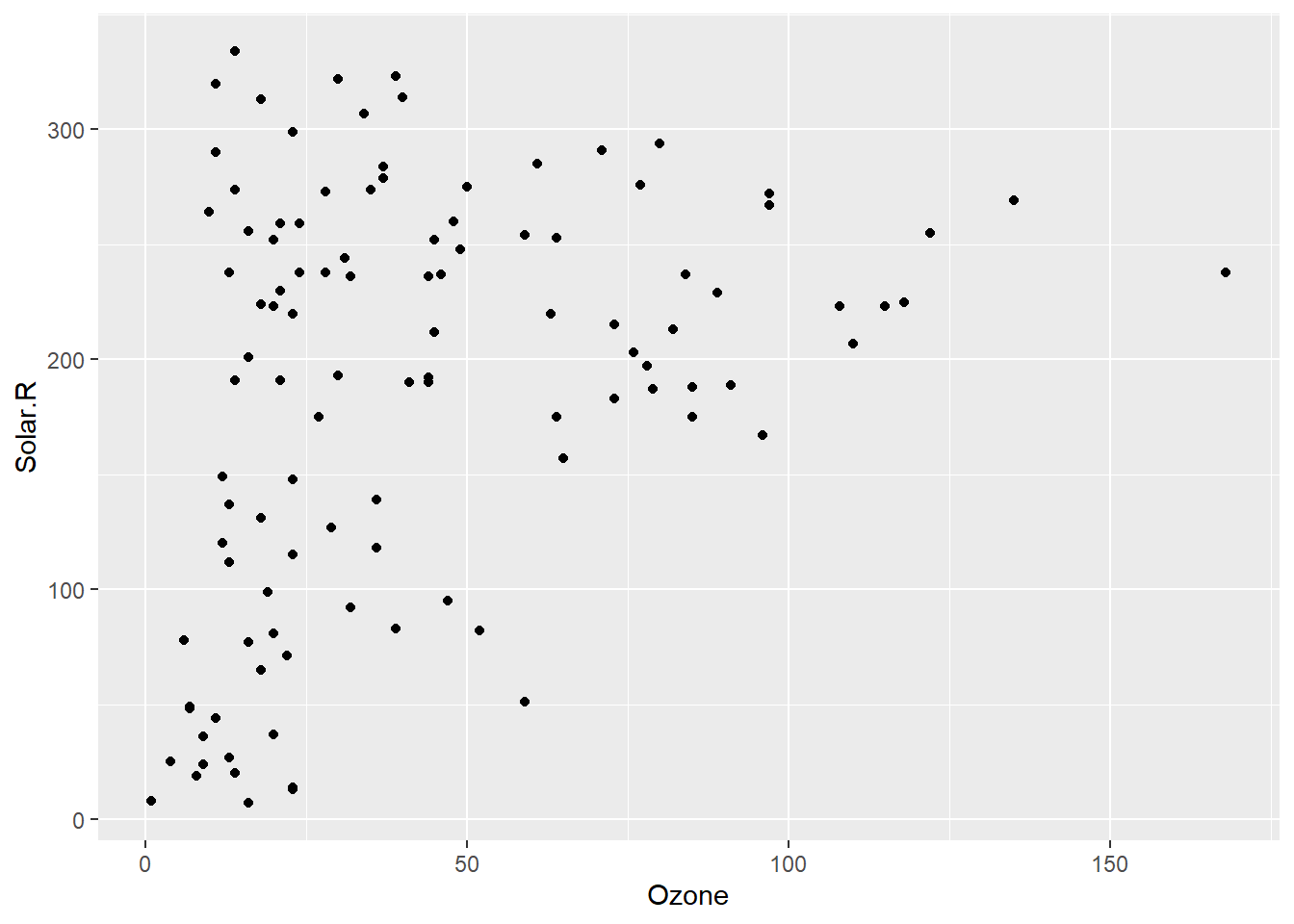
geom_miss_point allows those rows to be included in the plot. We can see the two observations missing both Ozone and Solar.R in the bottom left corner of the plot.
ggplot(airquality,
       aes(x = Ozone,
           y = Solar.R)) +
  geom_miss_point()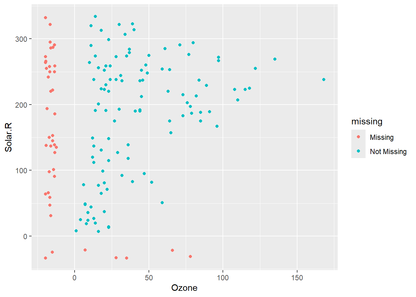
Missing data summaries
naniar also includes lots of special function to summarize the degree of missingness in different ways.
n_miss(airquality)[1] 44n_complete(airquality)[1] 874prop_miss(airquality)[1] 0.04793028prop_complete(airquality)[1] 0.9520697pct_miss(airquality)[1] 4.793028pct_complete(airquality)[1] 95.20697naniar contains many more useful features that you can explore [http://naniar.njtierney.com/articles/getting-started-w-naniar.html].
Shadow matrices
A shadow matrix is a simple way to keep track of which observations were originally missing. It augments the orignal data with a dataset of the same dimensions, where each cell is either “NA” or “!NA”. “NA” indicates that the value in that cell was missing in the original data, and “!NA” indicates that the value in that cell was not missing. One useful application of this is to visualize the quality of the missing data imputation.
aq_shadow <- bind_shadow(airquality)Missing data imputation
Missing data imputation is an advanced topic that requires careful study. Good references include (Enders 2010) and (Harrell 2016). When I need a simple, good-enough approach, I turn to the aregImpute function from the Hmisc package. This function:
- fits a flexible additive regression model to a bootstrap sample from the original data
- uses this model to predict all of original missing and non-missing values for the target variable
- for each missing value for the target or this revised report, variable, it uses predictive mean matching to identify the value among the non-missing values that has the closest predicted value
- uses the non-missing value of the closest match as the imputed value.
This approach has the advantage that it approximates using the full Bayesian posterior predictive distribution for imputation without having to specify a full Bayesian model, it has no trouble with collinear predictors, and it can naturally handle continuous, ordinal, and nominal variables (Horton and Kleinman 2007).
set.seed(1234)  # setting the seed for the random number generator, so the results are reproducible.

# generat a single imputed dataset from the aregImpute function
# there's nothing on the left hand side of the formula, so aregImpute will fill-in all columns with missing
# in this case, that's Ozone and Solar.R
# on the right hand side, we are specifying what data to use to fill-in the missing values.
# we are specifying that we want to use all 6 variables, which should give us the most information.
imputed <- aregImpute(~ Ozone + Solar.R + Wind + Temp + Month +Day, data = aq_shadow, nk = 0, n.impute=1)
Iteration 1
Iteration 2
Iteration 3
Iteration 4 #extract the imputation dataset from the imputed object created by the aregImpute object
impute1 <- impute.transcan(imputed, imputation=1, data=aq_shadow, list.out=TRUE,
pr=FALSE, check=FALSE)
#convert the impute1 list into a dataframe
completed <- data.frame(impute1)
#remove the "imputed" attribute from
attr(completed$Ozone, "imputed") <- NULL
attr(completed$Solar.R, "imputed") <- NULLYou can learn more about lists here and attributes here
We can see that the imputed values (teal) don’t stand out from the observed values (red), which is good! They are reasonable values.
#add back in the shadow matrix
completed_shadow <- cbind(completed, aq_shadow[,7:12])

# now plot the original and imputed values.
completed_shadow %>%
  ggplot(aes(x = Temp,
             y = Ozone,
             colour = Ozone_NA)) +
  geom_point()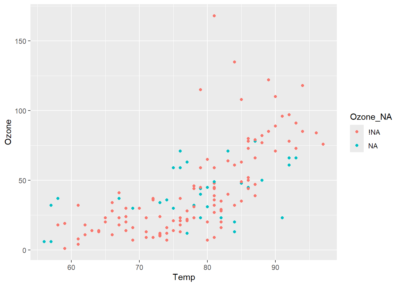
References
Enders, Craig K. 2010. Applied Missing Data Analysis. Guilford.
Harrell, Frank. 2016. Regression Modeling Strategies: With Applications to Linear Models, Logistic and Ordinal ... Regression, and Survival Analysis. Springer.
Horton, Nicholas J., and Ken P. Kleinman. 2007. “Much Ado about Nothing: A Comparison of Missing Data Methods and Software to Fit Incomplete Data Regression Models.” The American Statistician 61 (1): 79–90.